Detecting Outliers using the Boxplot Method

Outliers, the data points that diverge significantly from the overall pattern, can heavily influence the results of statistical analysis and make it challenging to draw accurate conclusions. Boxplot is one of the most effective and widely used methods to detect outliers in data.

Understanding Boxplots

A boxplot, also known as a box-and-whisker plot, is a graphical representation of data distribution using five summary statistics: minimum, first quartile (Q1), median (Q2 or the second quartile), third quartile (Q3), and maximum. The boxplot is divided into four sections, each representing 25% of the data points.

Steps to Detect Outliers Using a Boxplot

To detect outliers using boxplots, you can follow these steps:

1. Arrange the data in ascending order.
2. Calculate the first quartile (Q1), median (Q2), and third quartile (Q3).
3. Determine the interquartile range (IQR) by subtracting Q1 from Q3 (IQR = Q3 – Q1).
4. Calculate the lower and upper bounds for outliers. The lower bound and upper bound are included in the non-outlier zone.
   • Lower Bound = Q1 – 1.5 * IQR
   • Upper Bound = Q3 + 1.5 * IQR
5. Identify any data points that fall below the lower bound or above the upper bound as outliers.

Example 1

Given dataset: {22, 35, 2, 4, 20, 39, 37, 102, 101, 36}

Step 1: Arrange the data in ascending order: {2, 4, 20, 22, 35, 36, 37, 39, 101, 102}

Step 2: Calculate Q1, Q2, and Q3:

• Q2 (second quartile or median) = median({2, 4, 20, 22, 35, 36, 37, 39, 101, 102}) =(35+36)/2= 35.5
• Q1 (first quartile) = the median of the lower half (excluding Q2) = median({2, 4, 20, 22, 35}) = 20
• Q3 (third quartile) = the median of the upper half (excluding Q2) = median({36, 37, 39, 101, 102}) = 39

Step 3: Determine the IQR: IQR = Q3 – Q1 = 39 – 20 = 19

Step 4: Calculate the lower and upper bounds for outliers:

• Lower Bound = Q1 – 1.5 * IQR = 20 – 1.5 * 19 = -8.5
• Upper Bound = Q3 + 1.5 * IQR = 39 + 1.5 * 19 = 67.5

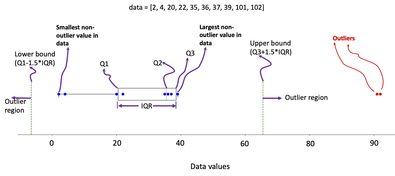
Step 5: Identify outliers: Any data points smaller than -8.5 or above 67.5 are considered outliers. In this dataset, we have two outliers: 101 and 102.

The following figure shows the corresponding boxplot.

Example 2

Given dataset: {28, 35, 1, 2, 4, 20, 20, 39, 37, 102, 101, 36}

Step 1: Arrange the data in ascending order: {1, 2, 4, 20, 20, 28, 35, 36, 37, 39, 101, 102}

Step 2: Calculate Q1, Q2, and Q3:

• Q2 (second quartile or median) = median({1, 2, 4, 20, 20, 28, 35, 36, 37, 39, 101, 102}) = (28+35)/2=31.5
• Q1 (first quartile) = the median of the lower half (excluding Q2) = median({1, 2, 4, 20, 20, 28}) = (4+20)/2=12
• Q3 (third quartile) = the median of the upper half (excluding Q2) = median({35, 36, 37, 39, 101, 102}) = (37+39)/2=38

Step 3: Determine the IQR: IQR = Q3 – Q1 = 38 – 12 = 26

Step 4: Calculate the lower and upper bounds for outliers:

• Lower Bound = Q1 – 1.5 * IQR = 12 – 1.5 * 26 = -27
• Upper Bound = Q3 + 1.5 * IQR = 38 + 1.5 * 26 = 77

Step 5: Identify outliers: Any data points below -27 or above 77 are considered outliers. In this dataset, we have two outliers: 101 and 102.

Example 3

The following video contains another example.

https://youtube.com/shorts/JyIAiK0jbMs?feature=share

Why does a boxplot contain a 1.5 IQR in the formulation?

The choice of using 1.5 times the interquartile range (IQR) as the threshold for detecting outliers in a boxplot is mainly based on statistical reasoning and practical considerations.

1. Statistical reasoning: The IQR represents the range within which the central 50% of the data points lie. By multiplying the IQR by 1.5, we create a range that covers approximately 99.3% of the data points in a normal distribution (assuming the data is normally distributed). This is based on the empirical rule or the 68-95-99.7 rule, which states that 68%, 95%, and 99.7% of the data fall within one, two, and three standard deviations from the mean. Since we use 1.5 times the IQR, we consider a range slightly wider than two standard deviations. Therefore, any data points outside this range are considered rare occurrences or potential outliers.
2. Practical considerations: The 1.5 IQR rule is widely used in practice because it balances sensitivity and specificity when detecting outliers. It is neither too strict (which would label many data points as outliers) nor too lenient (which would fail to identify real outliers). This makes it a practical and convenient choice for many applications, especially when dealing with moderate-sized datasets and in the absence of any domain-specific knowledge.

It’s important to note that the 1.5 IQR rule is a general guideline (when no other information/analysis is available) and not absolute. Different thresholds may be more appropriate depending on the nature of the data and the context of the analysis. For example, in some cases, using 1.5 IQR might be too aggressive, and a higher multiplier, like 2 or 3, might be more suitable for identifying outliers. Conversely, a lower multiplier might be needed to detect the outliers in other situations where the data is more prone to extreme values.

In summary, the 1.5 IQR rule is a good starting point for detecting outliers in a boxplot due to its statistical reasoning and practical considerations. However, (in a research environment), it is essential to understand the nature of the data and the context of the analysis to determine if this rule is appropriate or if a different threshold should be used.